How Eigen Vectors Are Used to Do Principal Component Analysis
Why Are Eigen Vectors Cool?
Eigen Vectors are so cool because they’re extremely useful in a lot of Engineering and Analysis applications. For one, they play a key role in Data Science by revealing hidden patterns in the data that tell you which data points are most significant. In this article we’re going to dive into a popular Data Science and Machine Learning technique, Principal Component Analysis.
Some Things We Need to Know About Linear Algebra and Matrix Multiplication First
Because obviously, we’re dealing with vectors, there are a few things we have to make sure we understand about vectors and Matrices (You can skip this section if you’re already familiar with those concepts)
Vectors
Ok, Quick recap on vectors, essentially, vectors are just lists of numbers. The amount of numbers in the list is what is referred to as the dimension. So for a vector like, [1, 3], we can say that it is 2 dimensional because there are two numbers in the list. If you’ve ever drawn any lines on an X, Y graph (remember, y=mx+b?), you’ve basically drawn a 2D vector. The same concept of course works for X, Y, Z graphs where you’d have 3 numbers in the vector, for example, 3D game graphics. Actually, vectors don’t really have a limit to how many dimensions they can be. You can have a 100 Dimensional vector if you want. Although us humans can’t really visualize graphs past 3D, it’s no problem at all for computers because the math still works the same way. The only real difference between drawing points on a graph and drawing vectors is that we usually think of vectors as being arrows that have a length and point in some direction. The length is usually referred to as the vector’s magnitude.
Matrices
Now that we understand what a vector is, it’s not really hard to conceptualize a matrix. A Matrix is just a list of vectors, packaged up into one unit. So if we had two vectors, for example [1, 3] and [2, 5], we can combine them together in a list, like this: [[1, 3], [2, 5]]. Now we have a 2 by 2 matrix. In matrix terminology, we call each vector in the matrix a row and each element of a vector a column. A common way to refer to the number of rows is with the letter n and for the for the number of columns, we use the letter m. So for example, if we have a matrix is 3 x 7, we can say that n is 3 and m is 7. So to summarize , a matrix is just a grid of numbers.
Matrix Multiplication
Ok, so now that we know matrices and vectors are just grids and lists of numbers, it makes sense that we should be able to do arithmetic on them. I won’t go into detail on every type of operation you can do with them, but in this post, we’ll just focus on multiplying a vector by a matrix. There are actually a few specific types of multiplication you can do with matrices and vectors, but the one we’re concerned with here is called the dot product. One important thing to note about the dot product is that is NOT commutative, which means A • B ≠ B • A. So the order you take the dot product matters, unlike normal multiplication where it doesn’t, like for example a * b = b * a. Here’s an example of how to take the dot product of a 3x3 matrix and a 3 dimensional vector:
[2 1 0]   [3]   [2*3 + 1*4 + 0*5]   [10]
[0 3 1] × [4] = [0*3 + 3*4 + 1*5] = [17]
[1 0 2]   [5]   [1*3 + 0*4 + 2*5]   [13]
The only stipulation in being able to multiple a matrix and vector is that the number of columns in the matrix must be match the number of elements in the vector. So let’s go back to our example of thinking of our vector, [1, 3], as a line on a 2D graph, drawn from the origin, [0, 0]. As long as some matrix has the same number of columns as the vector (in this case, two), we can multiply them and end up with a transformed vector. Transforming a vector just means taking the arrow it represents on the graph and changing its position, length, or orientation. The types of vector transformations are:
- Translation: Only changing the position (in this case away from the origin)
- Rotation around some axis
- Scaling (changing size)
- Shearing (skewing)
- Projection onto a plane or line (think of a shadow)
So when we multiply a matrix by a vector, we’re doing what is called a linear transformation, and the matrix is called a transformation matrix. So here’s the really interesting part; there are certain linear transformations you can do on a vector that scale its magnitude (length) without changing the direction it points in. Let’s go into a little more detail about what the significance of that is… because it’s pretty significant!
What Actually Are Eigen… things?
Ok aside from all the mathematical stuff, let’s get this out of the way… Who is Eigen? Well, Eigen isn’t a person (there are people with that name but they’re not really related to this topic). It’s just a German word that means "own," "inherent," or "characteristic." So I like to think about it as meaning the vectors that are kind of the “essence” of a particular linear transformation. So let’s image our X, Y graph again, but with points kind of ‘everywhere’ so they kind of make a grid representing a space. If we applied a particular linear transformation on that entire space, there could be some of those points that, if we thought of as vectors, don’t change rotation. They just scale into or out of a certain direction. Those vectors would be the eigenvectors of this specific transformation and the amount that they scale would be called the eigenvalues. So to recap, if we have a matrix we’ll call A and a vector we’ll call v, then we can express the concept of Eigenvectors as Av = λv where v is an Eigenvector and λ is the value that v is scaled by (we can refer to this as the scalar). Since λ, the scalar, scales the eigenvector, it is called the Eigenvalue. This is always true as long as our vector isn’t zero and the linear transformation doesn’t change the vector’s direction that it points in, only its magnitude (length).
To sum that up, the eigenvector is essentially the main characteristic vector of a specific linear transformation, as long as the vector is not zero (it wouldn’t have any direction in that case) and it’s direction doesn’t change, but just has it’s magnitude scaled. One more thing to note though. Eigenvalues can be negative so the direction can be reversed and it’ll still be ‘eigen’. This will be true as long as its angle doesn’t change. Oh, and one more thing, a linear transformation can have multiple Eigenvectors, they’re not limited to just one.
What Can You Do With Eigenvectors and Eigenvalues, What’s the Hype?
PCA - Principal Component Analysis
PCA is a really useful technique when you have data that has a lot of dimensions and you need to reduce it down to fewer dimensions. Doing this is called dimensionality reduction. Ok so why would you ever really need to do dimensionality reduction? One main reason is that data that is very high dimensional is difficult for humans to visualize and understand the meaning of. If you look at a graph that is 2D, it’s pretty easy to see how the different points on the graph relate to each other. If the graph is in 3D, it’s a bit more difficult, but being able to rotate that graph and view it from different angles makes it a bit easier. But what about 4D, 5D, etc.? Soon it becomes pretty much impossible to visualize and therefore understand what the data is telling you. This is where dimensionality reduction comes in. We can take some data that is, say for example 10 dimensional and reduce it down to 2D. Eigenvectors and Eigenvalues are the key players here because they let you sort of ‘shift your perspective’ of the data to view it from angles where the data varies the most. Using the ‘perspective’ analogy, the new ‘angle’ you’re viewing the data from is the way it looks when projected onto Eigenvectors that explain the most variance. We can find out which eigenvectors explain the most variance in the data by ordering them from largest to smallest in terms of their eigenvalues.
So how do you find the principal components of a dataset? If we were to do a matrix transformation on the space that our data lives in, any eigenvectors resulting from that transformation would be our principal components and the eigenvalues of those eigenvectors would denote which of the principal components explain which amounts of the variance in the dataset.
So, we know we need a matrix to do a transformation on the vector space to get our eigenvectors and eigenvalues. How do we decide what that matrix should be? The answer is, we use the covariance matrix of the data for this. Quick explanation of what a covariance matrix is though:
Covariance Matrix
So there are two distinct but closely related concepts to understand about Covariance Matrices. Covariance is the measurement of how the different values in one vector change in comparison to another vector of the same length. We’ll use the term Variance to explain how much the different values in a single vector differ with each other. In a covariance matrix, the values we see in the diagonal show us the variance in each particular vector. The numbers in each column tell us the covariance between its row’s vector and the vector whose variance is at that place in the diagonal. We can easily visualize this using a heat map with Seaborn in python like this:
import numpy as np
import seaborn as sns
import matplotlib as plt


thing1 = [38, 45, 32, 49, 89]
thing2 = [69, 2, 1, 67, 7]
thing3 = [18, 22, 3, 34, 68]

data = np.array([thing1, thing2, thing3])

covariance_matrix = np.cov(data, bias=True)

labels = ['thing1', 'thing2', 'thing3']

sns.heatmap(covariance_matrix, annot=True, fmt='g', xticklabels=labels, yticklabels=labels)

plt.show()
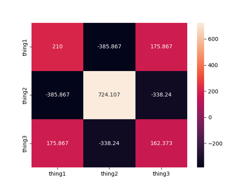
The variance of thing1 is X, the variance of thing2 is Y, and the variance of thing3 is Z. The Covariance of thing1 and thing2 is A The Covariance of thing1 and thing3 is B The Covariance of thing2 and thing3 is C
So, now that we have a covariance matrix and we understand what it means, we can use it to create a linear transformation over our vector space and see what the eigenvectors and eigenvalues are. BUT! We need to back up a bit and give our data a little treatment first. In this case, we’d probably be ok without doing it because we’re using made up data that kinda plays nicely with each other, but with real world data, we would likely have some values in the vectors that would grossly overshadow other ones. So to fix this we need to normalize the data first. There are a few ways to do data normalization, but here's we'll use a simple version of it called mean centering, which means we’ll ‘center’ the data by subtracting the mean value from all the features, like this:
mean = np.mean(data, axis=0) # get’s the mean (need to test this to make sure it works for matrices, if not I need to loop through each array)

mean_centered_data = data - mean # subtracts the mean from each point in the matrix
Now we can go back and plug our normalized data into the covariance matrix function so we can get a version of it that will give us a better representation of the covariances without really large numbers overshadowing smaller ones.
How Finding the Eigenvectors Actually Works
Now, to find the eigenvectors, we’ll first focus on finding one of them since we know all other possible ones will be orthogonal to that one if they exist. Remember, the formula for an eigenvector is Av = λv, So to find the first one, we will take the dot product of the transformation matrix, A with some vector, and if that vector’s direction doesn’t change, we’ll have an eigenvector. But wait… how do we ‘find’ an eigenvector? Should we just try random ones until we stumble upon one that doesn’t change direction? Luckily, there’s a much easier and more straightforward way to do it than that. All we have to do is start with any random vector in our vector space and multiply it by the transformation matrix recursively until it converges to an eigenvector. Ok, but why would it just magically ‘converge’ to an eigenvector? The reason is, the transformation matrix warps the entire vector space in the same way any time it is applied to a vector. So you can start with ANY vector in that space and keep feeding that result back in to be multiplied by the transformation matrix and every time you do, the result will be a new vector that points more and more in the direction that the transformation matrix is warping the vector space into. If you do this enough times, eventually the resulting vector will stop changing direction because it will be in the “Eigen” location of that vector space. So once you notice that it stops changing direction, you know you have your eigenvector. At that point, you can easily find the other eigenvectors because they’ll just be orthogonal to each other. Let’s look at how to do that without any libraries:
v = [1, 1, 1, ...] // or random vector
for i in range(max_iterations):
    v_new = A * v
    v_new = v_new / ||v_new||  // normalize

    if ||v_new - v|| < tolerance:
        break  // converged

    v = v_new
That’s just to illustrate how it works under the hood, but in practice we’d just use some libraries. Let’s look at how to put all that together and use Numpy to compute the covariance matrix, perform Eigen decomposition, sort the Eigen vectors by Eigen value, and finally project our original mean centered matrix onto the Eigen vectors to reduce their dimensions:
import numpy as np
import seaborn as sns
import matplotlib.pyplot as plt
import pandas as pd


# 3 vectors representing our data rows
thing1 = [38, 45, 32, 49, 89]
thing2 = [69, 2, 1, 67, 7]
thing3 = [18, 22, 3, 34, 68]

# create a matrix from vectors
data = np.array([thing1, thing2, thing3])

# mean center the data:
mean = np.mean(data, axis=0) # get’s the mean
mean_centered_data = data - mean # subtracts the mean from each point in the matrix

#----------------------------------------------------------------

# Compute the covariance matrix
covariance_matrix = np.cov(mean_centered_data, bias=True)

labels = ['thing1', 'thing2', 'thing3']

sns.heatmap(covariance_matrix, annot=True, fmt='g', xticklabels=labels, yticklabels=labels)

plt.show()

#----------------------------------------------------------------

# Perform Eigen Decomposition of the covariance matrix

eigen_values, eigen_vectors = np.linalg.eig(covariance_matrix)

print("eigen_vectors", eigen_vectors)
print("eigen_values", eigen_values)

#----------------------------------------------------------------

# Sort the eigen vectors in descending order of eigen values

indicies = np.arange(0, len(eigen_values), 1)
# zip pairs each eigenvalue with it's index, [::-1] reverses the list
indicies = ([x for _, x in sorted(zip(eigen_values, indicies))])[::-1]
eigen_values = eigen_values[indicies]
eigen_vectors = eigen_vectors[:, indicies]

print("sorted eigen vectors", eigen_vectors)
print("sorted eigen values",eigen_values)

#----------------------------------------------------------------

# Calculate the explained variance and select the top N components

eigen_values_sum = np.sum(eigen_values)
explained_variance = eigen_values / eigen_values_sum

print("explained variance", explained_variance)
cumulative_variance = np.cumsum(explained_variance)
print("cumulative_variance", cumulative_variance)

#----------------------------------------------------------------

# It's common to take the components with an explained variance of .95 or higher

# print highest k where explained variance is above .95

#----------------------------------------------------------------

# Take the dot product of our mean centered data and the eigen
# vectors to project the data onto those vectors

# transpose the original data so it's number of cols
# match the number of elements in the eigen vectors
pca_data = np.dot(mean_centered_data.T, eigen_vectors)

print("Transformed data ", pca_data.shape)

# plot the original data, mean centered, and transformed
That’s the basic idea behind using eigenvectors and eigenvalues to do principal component analysis. This post got a bit long, so I’m gonna save explaining the concept of Eigen Centrality to find the most important nodes in a network for the next post. Thanks for reading! Hope this helps make the concepts easier to grasp.
Discussion (0 Comments)